This post documents how I set up an NVIDIA CUDA GPU card on linux, specifically for CUDA computing (i.e. using it solely for GPGPU purposes). I already had a separate (AMD) graphics card I used for video output, and I wanted the NVIDIA card to be used only for computation, with no video use.

I found the whole process of setting up this card under linux to be problematic. NVIDIA’s own guidance on their website did not seem to work (OK, in fairness, you can sort of figure it out from the expanded installation guide pdf), and in the end it required patching together bits of information from different sources. Here it is for future record:

• Card: NVIDIA Quadro K1200 (PNY Low profile version)
• Computer: HP desktop, integrated graphics on motherboard (Disabled in BIOS - though in hindsight I don’t know if this was really necessary.)
• Linux version(s): Attempted on Fedora 23 (FAIL), Scientific Linux 6.7 (OK), CentOS 7.2 (OK). Officially, the installation scripts/packages only support Fedora 21, but I thought I would give it a try at least.

1st Attempt: Using the NVIDA rpm package (FAIL)

This is the recommended installation route from NVIDIA. Bascially you download the relevant package manager install package. I was using CentOS so downloaded the RHEL/CentOS 7 .rpm file. You then add this to your package manager (e.g. yum). For RHEL/CentOS, you must have the epel-release repository enabled in yum:

yum install epel-release

Then you add the rpm package downloaded from nvidia:

rpm --install cuda-repo<...>.rpm

Followed by:

yum clean expire-cache
yum install cuda

It will install a load of package dependencies, the CUDA package, as well as the proprietary NVIDIA drivers for the card. I rebooted, only to find I could no longer launch CentOS in graphical mode. It would hang when trying to load the X-server driver files on boot. Only a text interface login was possible. Further playing around with the linux system logs showed there was a conflict with some of the OpenGL X11 libraries being loaded.

I reverted to the earlier working state by launching in text mode and using yum history undo to revert all the installed packages in the previous step.

2nd Attempt: Using the NVIDIA runfile shell script (SUCCESS)

A second alternative is provided by NVIDIA, involving a shell script that installs the complete package as a platform-independent version. It bypasses the package manager completely and installs the relevant headers and drivers “manually”. NVIDIA don’t recommend this unless they don’t supply a ready-made package for your OS, but I had already tried packages for Scientific Linux/RedHat, CentOS, and Fedora without success.

Before you go anywhere near the NVIDIA runfile.sh script, you have to blacklist the nouveau drivers that will may be installed. These are open source drivers for NVIDIA cards, but will create conflicts if you try to use them alongside the proprietary NVIDIA ones.

You blacklist them by adding a blacklist file to the modprobe folder, which controls which drivers load at the linux boot-up.

vim /etc/modprobe.d/blacklist-nouveau.conf

Add the following lines:

blacklist nouveau
options modeset=0

Now rebuild the startup script with:

dracut --force

Now the computer has to be restarted in text mode. The install script cannot be run if the desktop or X server is running. To do this I temporarily disabled the graphical/desktop service from starting up using systemctl, like this:

systemctl set-default multi-user.target

Then reboot. You’ll be presented with a text-only login interface. First check that the nouveau drivers haven’t been loaded:

lsmod | grep nouveau Should return a blank. If you get any reference to nouveau in the output, something has gone wrong when you tried to blacklist the drivers. Onwards…

Navigate to your NVIDIA runfile script after logging in. Stop there.

Buried in the NVIDIA documentation is an important bit of information if you are planning on running the GPU for CUDA processing only, i.e. a separate, standalone card for GPGPU use, with another card for your video output. Theu note that installing the OpenGL library files can cause conflicts with the X-window server (Now they tell us!), but an option flag will disable their installation. Run the install script like so:

sh cuda_<VERSION>.run --no-opengl-libs

The option at the end is critical for it to work. I missed it off during one previous failed attempt and couldn’t properly uninstall what I had done. The runfile does have an --uninstall option, but it’s not guaranteed to undo everything.

You’ll be presented with a series of text prompts, read them, but I ended up selecting ‘yes’ to most questions, and accepting the default paths. Obviously you should make ammendments for your own system. I would recommend installing the sample programs when it asks you so you can check the installation has worked and the card works as expected.

After that has all finished, you need to set some environment paths in your .bash_profile file. Add the following:

PATH=$PATH:/usr/local/cuda-7.5/bin
LD_LIBRARY_PATH=$LD_LIBRARY_PATH:/usr/local/cuda-7.5/lib64

If you have changed the default paths during the installation process, ammend the above lines to the paths you entered in place of the defaults.

Now, you have to remember to restore the graphical/desktop service during boot up. (Assuming you used the systemctl method above). Restore with:

systemctl set-default graphical.target

Then reboot. It should work, hopefully!

Assuming you can login into your desktop without problems, you can double check the card is running fine, and can execute CUDA applications by compiling one of the handy sample CUDA applications called deviceQuery. Navigate to the path where you installed the sample CUDA programs, go into the utilities folder, into deviceQuery, and run make. You will get an application called deviceQuery that prints out lots of information about your CUDA graphics card. There are loads of other sample applications (less trivial than this one) that you can also compile and test in these folders.

Remember, if you have followed the above steps, you can only use your CUDA card for computation, not graphical output.

I run the LSDCatchmentModel (soon to be released as HAIL-CAESAR package…) on the ARCHER supercomputing facility on single compute nodes. I.e. one instance of the program per node, using a shared-memory parallelisation model (OpenMP). Recently, I’ve being trying to find the optimum setup of CPUs/Cores/Threads etc per node. (While trying not to spend too much time on it!). Here are some of the notes:

Compiler choice

I will write this up as a more detailed post later, but all these tests are done using the Cray compiler, a license for which is available on the ARCHER HPC. In general I’ve found this offers the best performance over the intel and gnu compilers, but more investigation is warranted.

The executable LSDCatchmentModel.out was compiled with the -O2 level of optimisation and the hstd=c++11 compiler flag.

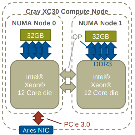
ARCHER compute nodes

Each node on ARCHER consists of two Intel Xeon processors, each with 32GB of memory. (So 64GB in total for the whole node, which either processor can access). Each one of these CPUs, with its corresponding memory, forms what is called a NUMA node or NUMA-region. It is generally much faster for a CPU to access its local NUMA node memory, but the full 64GB is available. Accessing the “remote” NUMA region will have higher latency and may slow down performance.

Options for Optimisation

Programs on ARCHER are launched with the aprun command, which requests the number of resources you want and their configuration. There are a vast number of options/arguments you can specify with this command, but I’ll just note the important ones here:

-n [NUMBER] - The number of “Processing Elements”, i.e. the number of instances of your executable. Just running a single 1 in this case.

-d [NUMBER] - The number of “CPUs” to use for the program. Here a CPU refers to any core or virtual core. On the ARCHER system, each physcial processor has 12 physical cores, so a total of 24 “CPUs” in total. I use “CPU” hereafter. With Intel’s special hyperthreading technology turned on, you actually get double the number of logical CPUs, so 48 CPUs in total.

-j 2 - Turns on hyperthreading as above. Default is off (-j 1, but no need to specify if you want to leve it off.)

-sn [1 or 2] the number of NUMA regions to use per program. You can limit the CPUS that are allocated to a single NUMA node, which may (or may not) give you a performance boost. by default processes are allocated on a single NUMA node until it is full up, then it moves on to the next one.

-ss “Strict segmentation’. Means that each CPU is limited to accessing the local 32GB of memory and cannot be allocated more than 32GB. If more than 32GB is needed, the program will crash.

-cc [NUMBER OR RANGE] CPU affinity, i.e. which CPUs to allocate to. Each logical CPU on the compute node has a number [0-23] or [0-47] with hyperthreading turned on. The numbering of CPUs is slightly counterintuitive. The first physical processor has CPUs [0-11] and [24-36] if hyperthreading is turned on. The second physical processor has CPUs numbered [12-23] and [37-48] if hyperthreading is turned on.

A typical aprun command looks like this: aprun -n 1 -d 24 -j 2 ./LSDCatchmentModel.out ./directory paramfile.params

Best options

ARCHER recommend to use only a single NUMA node when running OpenMP programs (i.e. don’t spread processes between physcial processors) but actually I have found for many cases, LSDCatchmentModel get the best performance increase from maxing out the number of CPUs, and turning on hyperthreading in some cases. There is not one rule, however, and different datasets can have different optimum compute node settings. For the small boscastle catchment, for example, running aprun -n 1 -d 48 -j 2 ... produced the fastest model run, which is contrary to what ARCHER recommend. (They suggest not turning on hyperthreading as well, for example.

OpenMP threads

OpenMP threads are not the same thing as CPUs. If you have 24 CPUs for example, your program will not automatically create 24 threads. In fact on ARCHER the default is just one thread! You can set this before you run aprun with: export OMP_NUM_THREADS=24 or however many you want. I haven’t really experimented with having different amounts of threads to availble CPUs, so normally I just set threads to the same number of CPUs requested with the -d option.

C++ can make use of native C libraries and header files. (As long as there is no incompatible stuff in the C implementation that will not compile as valid C++, there are only a few of these exceptions).

Example files

my_cpp_main.cpp
my_c_source.c
my_c_header.h

A normal #include "c_header.h" will not work, however. Instead use the extern keyword like so:

// normal C++ includes
#include <iostream> // or whatever...

extern "C"
{
  #include "c_header.h"
}

int main()
{
  call_some_func_c_header();

  // blah etc.
}

Then compile as follows:

g++ -c my_c_source.c my_main.cpp -o myExec.out

(remember to have the sources in the right order and before the executable!)

Some notes from the MPI course at EPCC, Summer 2016

MPI is the Message Passing Interface, a standard and series of libraries for writing parallel programs to run on distributed memory computing systems. Distributed memory systems are essentially a series of network computers, or compute nodes, each with their own processors and memory. The key difference between distributed memory systems and their shared-memory counterparts is that each compute node under the distributed model (MPI) has its own memory address space, and special messages must be sent between each node to exchange data. The message sending and receiving is a key part of writing MPI programs.

A very basic example: calculating pi

There are dozens of hello world example MPI programs, but these are fairly trivial examples and don’t really show how a real computing problem might be broken up and shared between compute nodes (Do you really need a supercomputer to std::cout “Hello, World!”?). This example uses an approximation for calculating pi to many significant digits. The approximation is given by:

where the answer becomes more acurate with increasing N.

The pseudo-code for the partial sum of pi for each iteration would be:

this_bit_of_pi = this_bit_of_pi + 1.0 / ( 1.0 + ( (i-0.5) / N)*((i-0.5) / N) );

For a basic MPI-C++ program, the first bit of the program looks like this, including the MPI header and some variables declared:

#include "mpi.h"
#include <iostream>
#include <cmath>

int main()
{
  int rank;
  int size;

  int istart;
  int istop;


  MPI_Status status;
  MPI_Comm comm;
  comm = MPI_COMM_WORLD;

  int N = 840;
  double pi;

  double receive_pi;
  // this is used for later computation of pi
  // from partial sums

  MPI_Init(NULL, NULL);

  MPI_Comm_rank(MPI_COMM_WORLD, &rank);
  MPI_Comm_size(MPI_COMM_WORLD, &size);

  std::cout << "Hello from rank " << rank << std::endl;

  //.. continues later

First, some variables are created to hold the rank, i.e. the current process, and the size, which is used to represent the total number of ranks, or processes.

istart and istop will be used to calculate the iteration loop counter start and stop positions for each separate process.

Secondly, the MPI_Status variable is defined, then the MPI_Comm type variable. These are special types defined in the MPI headers that relate to the message passing interface.

The MPI environment is initialised with MPI_Init(NULL, NULL);. The you can initialise the rank and size variables using the corresponding commands in MPI_Comm_rank() and MPI_Comm_size, passing a reference to the communicator object, and the respective variable.

By convention, the process with rank = 1 is used as the master process, and does the managing of collating data once it has been processed by the other ranks/processes.

The parameter N is used in our pi approximation and will determine the number of iterations we do. It is used to calculate the number of iterations distributed to each process:

  // Assuming N is exactly divisible by the number of processes
  istart = N/size * rank + 1;
  istop = istart + N/size -1;

Then each loop will calculate a partial sum of pi from its given subset of N. Because the MPI processes have been initailised, as well as the variables for rank and size, the code below will have unique values of istart and istop for each rank/process:

  // Check how the iterations have been divided up among 
  // the processes:
  std::cout << "On rank " << rank << " istart = " << istart \
            << ", istop = " << istop << std::endl;

  double this_bit_of_pi=0.0;
  for (int i=istart; i<=istop; i++)
  {
    this_bit_of_pi = this_bit_of_pi + 1.0 / ( 1.0 + ( (i-0.5) / N)*((i-0.5) / N) );
  }

  std::cout << "On rank " << rank << "Partial pi = " << this_bit_of_pi << std::endl;

Our partial sums have now been calculated, the last task is to collate them all together on the master process (rank=0), and sum them up:

  if (rank == 0) // By convention, rank 0 is the master
  {
    // take the value of pi from the Master's local copy of the 
    // partial sum
    pi = this_bit_of_pi;
    for (int source = 1; source < size; source++)
    {
      // Now we want to grab the parial pi sums from ranks
      // greater than zero (so start at source =1)
      int tag = 0;

      MPI_Recv(&receive_pi, 1, MPI_DOUBLE, MPI_ANY_SOURCE, tag, comm, &status);

      std::cout << "MASTER (rank 0) receiving from rank " << status.MPI_SOURCE \
                << std::endl;

      // Now add to received partial sum to the running total
      pi += receive_pi;
    }
  }

The key part of the above code is that we are telling the master process (rank=0) to be ready to receive all the partial sums of pi. MPI requires both send and receive calls. However, the send command has to be issued from the respective processes themselves (There’s no ‘get’ command per se, it’s a two-stage process that has to be set up on each process correctly).

Now we tell the non-master processes to send their partial pi sums:

  else // i.e. else not rank=0...not on the master process
  {
    // Now send the other partial sums from each process to the master
    int tag = 0;

    std::cout << "Rank " << rank << " sending to rank 0 (MASTER)" << std::endl;
    // Use a synchronous send (Ssend)
    MPI_Ssend(&this_bit_of_pi, 1, MPI_DOUBLE, 0, tag, comm);
  }

So now we’ve issued a command to send all the bits of pi, specified the data type, MPI_DOUBLE and passed the other arguments required by MPI_Ssend().

Finally, we can do the last bit of the calculation needed in the original formual by multiplying by four. Then finalise the MPI processes.

  pi = pi * 4.0/(static_cast<double>(N));

  MPI_Finalize();

.

The full program is given in a github Gist, which I will either embedd or provide a link to soon.

Writing a simple Python wrapper for C++

I wanted to write what is essentially a wrapper function for some C++ code. Looking around the web turned up some results on Python’s ctype utility (native to Python), the Boost::Python C++ libraries, and the Cython package, which provides C-like functionality to Python. I went with Cython in the end due to limtations with ctypes and warnings about magic in the boost library.

The Cython approach also is completely non-interfeing with the C++ code – i.e. you don’t have to go messing with your C++ source files or wrapping them in extern “C” { }-type braces, like you do in ctype, and strikes me as a awkward to go around modifying your C++ code.

You need to have the Cython and distutils modules installed with your Python distribution for this. Examples here use Python 2.7, but there’s no reason I know of why Python 3.x won’t work either.

The C++ program

For this example, I’m using a little C++ program called Rectangle.cpp which just calculates the area of a rectangle from a Rectangle object. The example is basically lifted from the Cython docs, but the explanation is padded out a bit more with working scripts and source files. (Unlike the cython.org example which I found almost impossible to understand)

Rectangle.cpp

#include "Rectangle.hpp"

namespace shapes 
{ 
  Rectangle::Rectangle(int X0, int Y0, int X1, int Y1) 
  { 
    x0 = X0; y0 = Y0; x1 = X1; y1 = Y1; 
  } 
  Rectangle::~Rectangle() { } 
  
  int Rectangle::getLength() { return (x1 - x0); } 
  int Rectangle::getHeight() { return (y1 - y0); } 
  int Rectangle::getArea() { return (x1 - x0) * (y1 - y0); } 
  void Rectangle::move(int dx, int dy) { x0 += dx; y0 += dy; x1 += dx; y1 += dy; }
}

Rectangle.hpp

namespace shapes 
{ 
  class Rectangle 
  { 
    public: int x0, y0, x1, y1; 
    
    Rectangle(int x0, int y0, int x1, int y1); 
    ~Rectangle(); 
    
    int getLength(); 
    int getHeight(); 
    int getArea(); 
    void move(int dx, int dy); 
  }; 
}

The Python (and Cython) files

From the python side of things, you’ll need 3 files for this set up:

1. The rectangle_wrapper.pyx cython file.
2. The setup.py file.
3. For testing purposes, the test.py file.

The Cython file rectangle_wrapper.pyx is the Cython code. Cython code means C-like code written directly in a Python-like syntax. For this purpose, it is the glue between our C++ source code and our Python script which we wantto use to call the C++ functions. The Cython file is a go-between for Python and C++.

The setup.py file will handle the compilation of our C++ and Cython code (no makefiles here!). It will build us a .cpp file from the Cython file, and a shared library file that we can import into python scripts.

rectangle_wrapper.pyx

#This is a Cython file and extracts the relevant classes from the C++ header file.

# distutils: language = c++
# distutils: sources = rectangle.cpp

cdef extern from "Rectangle.hpp" namespace "shapes":
    cdef cppclass Rectangle:
        Rectangle(int, int, int, int)
        int x0, y0, x1, y1
        int getLength()
        int getHeight()
        int getArea()
        void move(int, int)

cdef class PyRectangle:
    cdef Rectangle *thisptr      # hold a C++ instance which we're wrapping
    def __cinit__(self, int x0, int y0, int x1, int y1):
        self.thisptr = new Rectangle(x0, y0, x1, y1)
    def __dealloc__(self):
        del self.thisptr
    def getLength(self):
        return self.thisptr.getLength()
    def getHeight(self):
        return self.thisptr.getHeight()
    def getArea(self):
        return self.thisptr.getArea()
    def move(self, dx, dy):
        self.thisptr.move(dx, dy)

setup.py

from distutils.core import setup
from distutils.extension import Extension
from Cython.Distutils import build_ext

setup(ext_modules=[Extension("rectangle_wrapper", 
                             ["rectangle_wrapper.pyx", 
                              "Rectangle.cpp"], language="c++",)],
      cmdclass = {'build_ext': build_ext})

You now have all the files needed to build the module. You can build everything using the setup.py script by doing: python setup.py build_ext --inplace

This generates two extra files: the .cpp source code file and the linked library file (.so in linux.) You can now run the test.py file below or experiment with the module in an interactive console. Note that this does not install the module into your python installation directory – you need to run the script from the same directory as your linked library files, or add the directory to the pythonpath.

test.py

#Note how you can just import the new library like a python module. The syntax in the Cython file has given us an easy to use python interface to our C++ Rectangle class.

import rectangle_wrapper

# initialise a rectangle object with x0, y0, x1, y1 coords
my_rectangle = rectangle_wrapper.PyRectangle(2,4,6,8)

print my_rectangle.getLength()
print my_rectangle.getHeight()
print my_rectangle.getArea()